General workflow
In every update of DGM-deep, new available public data is incorporated based on a workflow, captured in scripting. A limitation of the method applied however, is that it results in a simplified representation of structural complexity, particularly around salt structures and reverse faults. A duplication in stratigraphy as is the case near overhanging salt structures or reverse faults, for example is simplified to a sub-vertical representation.
The applied modelling workflow includes the interpretation of horizons from 3D and 2D seismic data in the time domain (two way travel time). Stratigraphic markers interpreted in wells with time and depth information help to identify horizons in the seismic data. Time grids result from interpolation of seismic horizon picks using a gridding algorithm (convergent gridding). Subsequently, a conversion to the depth domain is made using a velocity model built from well log and checkshot data.
After time-depth conversion, per layer, the misties of each surface grid with the well marker depths are analyzed. Abnormally high misties caused by e.g. the simplified representation of complex features in the model output, are filtered out or used for a local correction. After analysis of the misties a subset of wells per stratigraphic layer remains, which is used for well correction in depth. The number of wells in the residual (mistie)-selection also differs for each stratigraphic layer because they strongly depend on the lateral extend of the unit and the end depth of the well. After analyzing the misties a varying selection of ca. 600-3500 wells have been used for correcting the depth horizons.
For each horizon the mistie values are interpolated with a kriging algorithm. The resulting well residual grids are combined with the time-depth converted grids to obtain a well-tied stratigraphic model, i.e., that acknowledges the well data (see also Kombrink et al., 2012). In a final step the models’ uncertainty is addressed by calculating standard deviation grids resulting from stochastic simulations of those horizons that are based on seismic interpretation.
Kombrink et al., 2012 (PDF, 7,94 MB) NJG
Publication of the offshore DGM-deep, modelling workflow and -results.
Explanatory note uncertainty(PDF,322 kB)
Description of uncertainty procedure DGM-deep
Nomenclature Deep
Online reference-book of the lithostratigraphic units of the deep subsurface of the Netherlands. The Table in the online Stratigraphic Nomenclature of the Netherlands illustrates lithostratigraphic units at group level in a schematic representation of the Geological timescale.
Overview of the modelled units in DGM-deep v5.0 (PDF, 90 kB)
Legend of the modelled units included in the visualisations of this portal. Saving visualisations is explained in the FAQ.
Model updates DGM-deep v5.0
In the DGM-deep v5.0 model the following updates were incorporated.
- In DGM-deep v5.0 models of the onshore and offshore are combined into one model. The on- and offshore models were modeled in the projection system of the input data. To merge both models the onshore model, modeled in the projection system RD-Bessel 1841, has been converted to projection system ED50_UTM31, and subsequently merged into one model. In support of studies in the Dutch onshore area only, it is advised to use the onshore model in the projection system RD-Bessel 1841 (Note: additional comments in sections below for the Rotliegend Group and Limburg Group).
- New time interpretations of the Upper-Germanic Trias Group (RN) in onshore areas covered by 3D surveys have been included in the model. Interpolation of the horizon interpretation and time-depth conversion has only been executed for these 3D-data areas. Because the Upper-Germanic Trias Group in onshore 2D-surveys has not been interpreted, the 2D-areas have been modelled using well data.
- The onshore time model has been depth converted with the VELMOD-3.1 velocity model. This update of the VELMOD-model has been disseminated in 2018 (More information Van Dalfsen et al., 2006 (PDF, 2,14 MB) and VELMOD1-3.1).
- Time horizons have been clipped at pre-defined layer boundaries and merged into one compiled, coherently stacked, model in the time domain. These layer boundaries, which were defined in previous studies (DGM-deep v1.0 – v4.0), have been revisited and edited in the time and/or depth domain. For example, edits have been applied to areas with well data indicating the presence of a stratigraphic layer and a layer thickness below seismic resolution. In these cases the pre-defined layer boundaries of the time model have been extended to also include these wells and to match well depth at these locations (a.o this applies to the Chalk Group in the Broad Fourteens Basin). In DGM-deep v5.0 it was not possible to solve all issues with wells outside horizon boundaries. In a future release this will be re-addressed.
- In DGM-deep v5.0 initially all non-confidential wells from the DINO database were used in the analysis of misties between mapped horizons and well marker depth. A cutoff value of less than +/- 10% compared to well depth has been applied as a primary selection criterium in the mistie selection. The resulting number of wells selected for well correction per stratigraphic layer is: NU = 1641, NL+NM = 3539, CK = 2683, KN = 2740, S = 778, AT = 588, RN = 1016, RB = 1518, ZE = 1830). In the well-residual selection process a number of wells unintentionally have been excluded from the selection of misties. This is the case for wells from the area of the Texel IJsselmeer High, the Zeeland High, and in the eastern part of the Peel-Maas Bommel Complex. In these areas no mistie correction was applied.
- The base of the Upper Rotliegend Group has been modeled by calculating a thickness grid based on welldata, which subsequently was added to the base of the Zechstein Group. This calculation and the resulting thickness grid was based on one well-data set for the on-and offshore in the projection system ED50-UTM31. Results are only published in the Projection system ED50-UTM31.
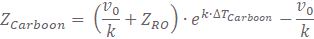
- The bases of the Limburg Group (DC) and Caumer subgroup (DCC) are available in the projection system RD-Bessel 1841. The base of the Limburg Group (DC) has been re-interpreted in the SCAN-Dinantian project. Results can be retrieved via the Dinantian mapping results webpage. The base of the Caumer subgroup (DCC), published in the DGM-deep v5.0 model dataset, is only covering the onshore area. The Interpretation of DGM-deep v4.0 of the Caumer subgroup has been incorporated without changes in the modeling process of DGM-deep v5.0. The SCAN-Dinantian report describes the velocity model (in this case with constant values for v0 and k), which is used for time-depth conversion of these carboniferous horizons. To successfully perform time-depth conversion, a reference level in depth and time is needed. In this case the base of the Rotliegend Group has been used as a reference. Because this horizon is not seismically based, no time grid is available. To obtain the base of the Rotliegend Group in time, a time thickness has been calculated using velocity information and the Rotliegend thickness grid. In turn, time thickness of the Limburg Group (∆TDC) and of the Hunze-Dinkel-Caumer subgroepen (∆TDCH+DCD+DCC) can be calculated using the calculated base Rotliegend Group time horizon as top horizon. Subsequently the following formula was used to depth convert the base Carboniferous horizons (see SCAN-Dinantian report for further details).
- For consistency in visualization in the subsurface viewer and in x-sections of the dinoloket x-section tool, the bases of the Limburg Group (DC) and Caumer subgroup (DCC) have been modified; In the visualizations these horizons show a grid coverage somewhat different compared to the disseminated depth grids. Coverage of DC and DCC depth grids are based on coverage and quality of available seismic data. Depth grids show “no-data” areas for large areas offshore, South Limburg, and several areas in the center and north of the Netherlands onshore. Grids visualized in the subsurface viewer are continuous in the “no-data” areas in the center and north of the Netherlands onshore. A smoothed Rotliegend base grid was used as trend-grid in steering interpolating of these gaps in the grids. Furthermore, the entire offshore area has been omitted in the visualizations.
- DGM-deep v5.0 offshore depth grids have been harmonised with offshore depth grids of the United Kingdom. The UK-grids have been published by the British Oil and Gas Authority (OGA) and can be retrieved from the OGA website “OGA and Lloyd’s Register SNS Regional Geological Maps”.